Data Normalization, Geocoding, and Error Assessment

GOALS AND OBJECTIVES

The goal of this lab was to explore geocoding. Geocoding involves using software to match up location descriptions, such as addresses, to actual coordinates on the Earth's surface. In order to geocode, the data had to be sufficiently normalized. This was done by manipulating tables to create similar data for each entry in the table. After geocoding and manual cleanup, error assessments were made to analyze the success of the process.

This lab served as a continuation of the previous frac mining labs. This meant that the data used was frac mine locations, whose locations were given as addresses or described with PLSS. The results from this lab will be used in subsequent labs using network analysis.


METHODS

Before the data could be used in any meaningful way, it had to first be normalized. The goal of normalization is to have a uniform style of data entry so data could easily be compared and analyzed. The initial spreadsheet used is shown below in figure 1. All the location data is given in a single column. Notice the variety of location descriptions. There is PLSS descriptions mixed with addresses. Some have both or only one, and there is no uniform method of entry.

Figure 1: Data before normalization

To normalize the data, entries were split into separate columns: an address column and a PLSS column. This is shown below in figure 2. The geocoding software uses addresses only, so PLSS data would just be for manual cleanup after the geocoding had been run.

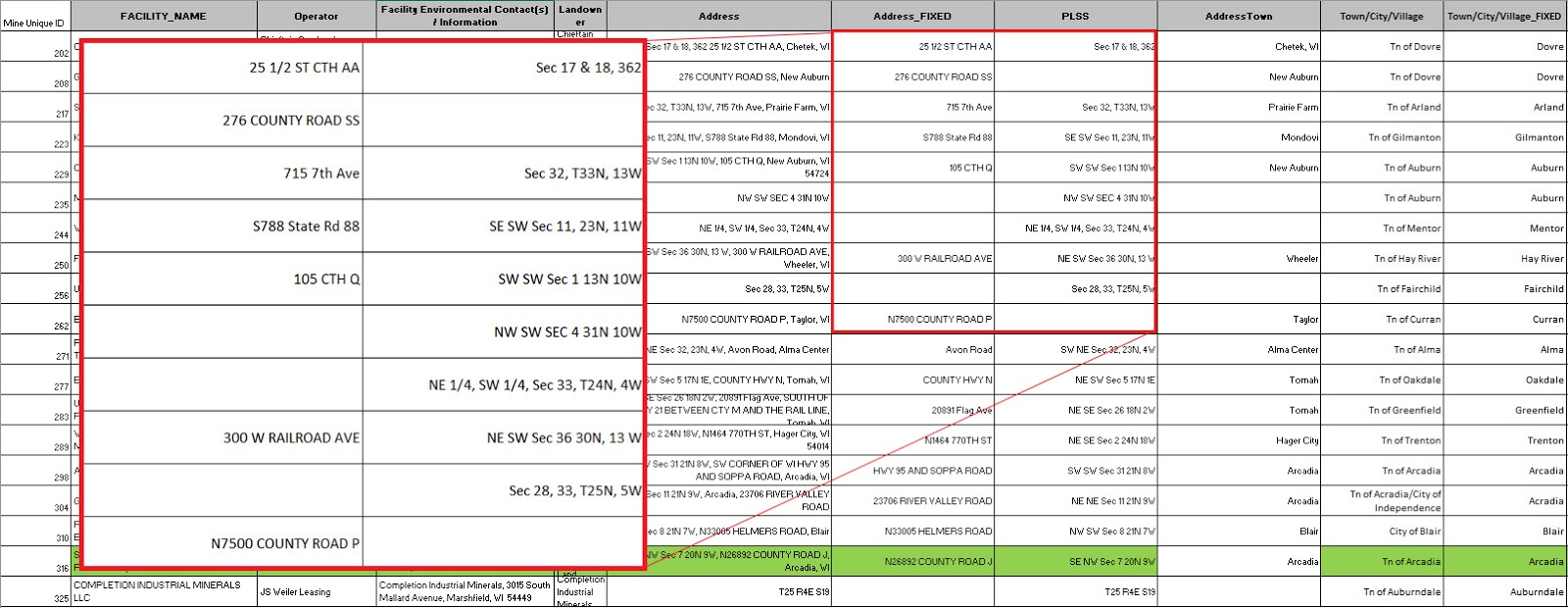Figure 2: Data after normalization

With the data normalized, it was ready to be geocoded. The spreadsheet was brought into the geocoding tool on ArcMap. This tool analyzed the address and town fields to find possible matches for locations. This could only be done on entries with addresses given. For entries with only PLSS locations, the estimated location was automatically chosen at the center of the given town. A visual of this process is shown below in figure 3. First the PLSS township was found, as shown on the right. In this example, the PLSS township was 33 N 13 W. Next, the subsection was used, as shown in the middle. This mine was described as being on the border of section 29 and 32. The area was searched for a mine and found, as shown on the right. The location, as marked by an X, was placed on the road to ease in network analysis for future labs.

Figure 3: Using PLSS data to find mine locations

This was done for all mines with PLSS data. All other mines were similarly checked to make sure the location was marked at the entrance of the mine. Many of these were off and had to be manually corrected, as the geocoding software uses approximations to guess locations for addresses.

For error analysis, the data was compared to both the class's data and the coordinates given by the data provider. Comparisons were made in a similar way for each. For comparisons to student data, all mine shapefiles were merged into a single feature class and projected in in Central Wisconsin State Plane projection. The lab was designed so there was overlap enough so each mine was located by several students. This meant the feature class had multiples of the same mines. Once this feature class was created, a model was made to split each unique mine into separate feature classes. This model is shown below in figure 4. The model iterates through the feature class containing all mines and groups mines with the same mine ID into their own feature classes, naming each output file by the unique mine ID. This was done so each student mine locations could be compared to the corresponding mine location I found. These distances would be averaged to find average distances between my mines and mine locations found by others.

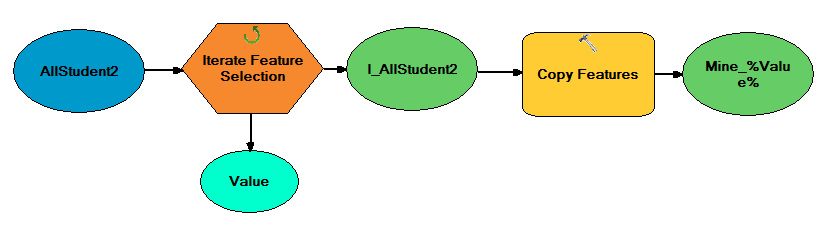Figure 4: Model created to split unique mines into separate feature classes

This same process of splitting to individual mines was used to the shapefile of actual mine locations given by the DNR. In this case, however, there was a one-to-one ratio of mines being compared, as I was not using data from multiple people.

After error analysis was completed, maps were created showing the comparisons of mine locations I found to locations found by other students and to those given by the DNR.


RESULTS

The error calculations performed are shown below in figure 5. Notice there are many more mines being compared under student mines because there were several instances of each mine compared. The averages, or average distance between my mine and other mines, were both around 1700 m.

Figure 5: Error calculations

Shown below in figure 6 is the map created comparing my mine locations to those of other students. Notice that many mines overlap, some completely. There are some outliers, however. Most of these are from a student choosing the wrong mine in the area.

Figure 6: Comparison of my mine locations to those found by students

Shown below in figure 7 is the comparison of my mines to the "actual" locations given by the DNR. I hesitate to call them that because many of these DNR locations have low precision, and are placed a distance from where the mine is clearly located on aerial imagery. This is a cause of higher error found previously.

Figure 7: Comparison of my mine locations to those given by the DNR

DISCUSSION

Using the model turned out to be an excellent way to efficiently split feature classes for easier use. Doing this allowed me to compare all mines available rather than taking a sample and only comparing 10 or 20 percent of the mines.

There are a few sources of error that make the average distances non-zero. One is that not all mines analyzed are active. Some mines are closed and reclaimed as vegetated areas, with makes their precise location difficult to assess. For these, maps from different temporal resolutions were used. Some mines, however, were only permitted and construction had not yet begun. There was no real way to find precise locations on these, so locations were marked near open areas away from private residences. There were some mines that were found, but were large and had multiple entrances. This resulted in the lower end averages that are seen, as some students picked a different entrance than I. There were some instances of choosing the wrong mine, as some areas have a high density of mines and only have a vague PLSS description of the mine location, resulting in ambiguity of which mine is the correct one.


CONSLUSION

Geocoding is a powerful tool that is used by almost everyone. Typing an address into Google to find its location is an example of how geocoding is used in every day life. Geocoding as an analysis tool proved to be extremely useful, but not without its shortfalls. A significant amount of time was spent checking and correcting mine locations from either incorrectly estimated locations or the inability for the software to use PLSS location data. Nevertheless, the geocoding software has impressive abilities that become most useful when dealing with a large number of data entries. The amount of time it takes to locate entries with geocoding software is a fraction of the time it would take manually.