This lab explores network analysis tools. Network analysis uses networks, in this case road networks, to model routes, distances, and travel times. Whereas traditional analysis uses straight lines, "as the crow flies" routes, from one point to another, network analysis can more accurately analyze how far and how long it takes to travel between points. The tool has a wide range of applications, from routing emergency vehicles on the quickest path, to modeling waterway networks, to finding travel routes around construction zones. Applications of this network analysis are widespread.
In this lab, the sand mine data used previously will be studied here. The goal of this lab is to find hypothetical costs associated with road wear caused by heavy mining vehicles using public roads. To do this, routes must be established that the vehicles will take, then the distance of these routes needs to be determined, followed by the total cost calculated from this distance.
METHODS
This lab began with a Python script (can be viewed here under script 2) that used SQL queries to find mines that would need to use roadways to transport frac sand. This was done by removing deactivated mines and mines that are connected to a rail terminal. Next, the script used a select by location to remove mines that were 1.5 km from a rail terminal, as these would have spurs built that would eliminate the need for roadway transport. The script was run and the relevant mines were extracted successfully.
These mines were then brought into ArcMap, along with rail terminal locations and road network analysis features. To minimize error, the network analysis was then done with a model. This model is shown below in figure 1. The three inputs: streets, mines, and rail terminals were used in the network analysis tool to find the closest route from each mine to a rail terminal. These calculated routes were copied and exported to a new feature class. A map showing these routes can be seen in the results section.
 |
| Figure 1: Model created for network analysis |
Next, a model, shown in figure 2, was used to estimate the hypothetical cost that vehicles using the routes would incur on roadways. The cost was estimated per county. First, in the model, the routes were projected to a Wisconsin HARN projection to minimize distortion. next, the routes were cut along county lines with the identity tool. This was done so distance calculations within counties would be limited to sections of routes that fall within the county. The identity tool added fields to the routes that had data on which county each section of the route was in. The summary statistics tool then merged all route sections by county to determine total distance of route in each county. Add and calculate field tools were then used to take this distance, convert it into miles, multiply this by a hypothetical cost of 2.2 cents per mile and 50 trucks making a round trip per year. The numbers used are hypothetical and could be easily changed by altering variables in the model.
 |
| Figure 2: Model created to estimate cost per county for road usage |
RESULTS AND DISCUSSION
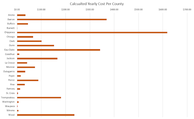
Shown below in figure 3 are the routes that were predicted from each mine a rail terminal. Notice there are some rail terminals that connect to multiple mines. Also, overlapping routes are still considered to be separate routes, so distance is calculate individually per route. This is why, as will be shown in the cost calculations, counties with a dense network of routes have a higher predicted cost than counties with a single, long route.
 |
| Figure 3: Routes from mines to rail terminals |
Below in figure 4 is a chart showing estimated costs per county. This was created by exporting the table created by the second model to Excel. There are many counties with negligible calculated costs as a route only briefly passes through. The counties with the highest costs have dense networks of predicted routes. The calculated costs for roadway wear were relatively low compared to the scale and cost of sand mine operations. Of course, the cost per mile, one of largest factors, was just a hypothetical estimate in this exercise and the actual cost per mile could be much higher or lower.
 |
| Figure 4: Chart showing hypothetical yearly costs per county |
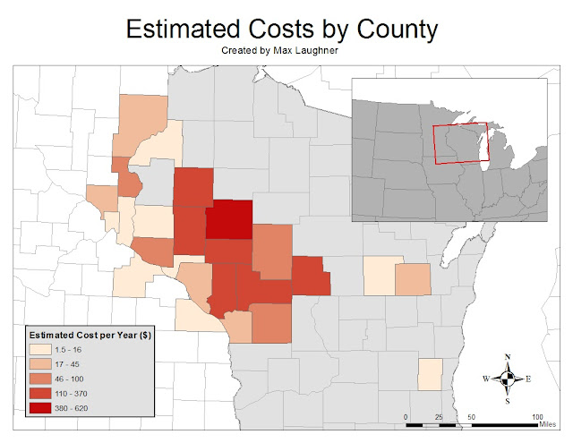
Lastly, shown in figure 5 is a map depicting estimated costs by county.
 |
| Figure 5: Map showing hypothetical yearly cost per county |
There are many assumed variables that cause uncertainty in this estimation. Beyond the hypothetical values used for estimating cost, the method of analyzing routes should be considered. The model chose the route that takes the least amount of time. This may not be accurate, as in reality, routes would also be directed away from high-traffic areas, along with other factors. These factors can be assessed with the network analysis tool with access to pertinent data.
CONCLUSION
Network analysis is a robust tool with widespread applications. Despite this, the tool is relatively easy to use and adapt to fit the application. As shown in this lab, the results from the tool can easily be used in conjunction with other tools as needed. While specialized uses for network analysis, such as cost estimations, are common, even more common is its use in personal routing. Entering a location into Google Maps, for example, uses network analysis to determine the most efficient routes to take. The usefulness of network analysis cannot be stressed enough.
No comments:
Post a Comment