Tuesday, May 16, 2017

Raster Analysis

GOALS AND OBJECTIVES

This lab explored raster functions in the context of frac sand mining in Trempealeau County. Raster functions are powerful tools with a wide range of functions. These functions were used to determine suitable land for frac sand mines and land where mines may have a high environmental impact both considering a variety of factors. Using these findings, areas of high mine suitability with low negative impact were located. Note that only the southern portion of Trempealeau County was considered to cut down on processing time.


METHODS

First, geoprocessing environments were set up to only analyze the study area. Cell size defaults for rasters were set to 30 x 30 meters to ensure data integrity. A mask was used in the environment so all rasters created would have the same extent of lower Trempealeau County.

Land Suitability

To find areas suitable for sand mines, a variety of factors were considered. These included geologic, land use, distance to railroads, low slope, and water table requirements. For each factor, land was ranked on a scale for how suitable it was based on each factor. This is outlined in the table below in figure 1.

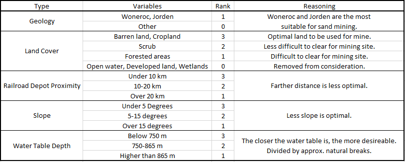
Figure 1: Suitability factors

Geology was based on whether the geology type was Woneroc or Jorden, which are the most suitable for mining. Geologies of these types were extracted as a raster.

Land cover uses were judged on a scale, where clear, open lands were the most suitable. The more difficult it is to clear an area, the less suitable the land was. Devloped land and open water were removed from consideration completely. The types were extracted as rasters

Next, railroad depot proximity was considered. The farther a mine is from a railroad depot, trucks will have to travel farther to drop off product. Areas closer to depots were given a higher suitability rank. Euclidean distance to railroad depots was calculated and the distances were ranked in a raster.

Next, slope was considered. Lower slopes would be considered optimal, as it would be easier to traverse the mine site with the necessary heavy equipment. Lower slopes were ranked as more suitable. Slope was extracted from a county DEM. A filter was used to remove some of the salt-and-pepper effect this produces. Slopes were reclassified to be ranked.

Lastly, water table depths were considered. Since mines use water in the mining process, it would be optimal to procure water at the site. The deeper the water table is, the more difficult that would be, thus deeper water tables were ranked as less suitable. Contours of water table depths were used to create a depth raster. These depths were reclassified to judge suitability.

Once the rasters for each factor were ready, a model was created to build an overall suitability raster. The model created is shown below in figure 2. The Raster Calculator SQL is as follows:

("%Geol_Suitable%" + "%NLCDreclass%"  +  "%RailDistFinal%" + "%SlopeSuitabilityFILTER%" + "%WTDsuitability%") * "%NLCDexclude%"

The SQL adds the factors together and multiplies this result by the exclusion areas. The areas excluded have a value of 0, with all other area having a value of 1 within the exclusion raster. This replaces the rank of excluded areas with a null value.

Figure 2: Model created for land suitability factors


Environmental and Social Impact Consideration

Solving for impact factors was completed in using the same workflow. The factors considered were impacts to streams, prime farmland, residential areas, schools, and trails. Once again, each factor was assigned a rank as shown below in figure 3. The higher the rank, the more impact the variable had.

Figure 3: Impact factors
Mines can impact streams from water contamination. The greater the distance to a stream, the less contamination will occur. This is a slight simplification, as there are many other variables that can determine this. For the scope of this lab, however, only Euclidean distance was considered. A vector of rivers within the county was used for this. Since streams and rivers are ubiquitous in Trempealeau, only major rivers of order 3 and up were considered. These were extracted with a simple SQL query. From this extracted vector, the Euclidean Distance function was used to determine distance from these rivers. From here, distances were reclassified to assign ranks.

To avoid placing a mine on prime farmland, farmland data was used. This came as a vector which classified land's suitability for farmland. This polygon vector was converted to a raster and the suitability of farmland was ranked.

Next, residential impacts were assessed. Land use data was procured from the Trempealeau County Geodatabase. From here, land with residential use was extracted through a query. From here, the Euclidean Distance tool was used to determine distance from residential land. Zoning laws dictate that mines cannot be within 640 meters from residential properties. The farther they are, the lesser the noise and dust impact would be. These distances were ranked as a raster through the Reclassification tool.

For similar reasons to residential land, schools should also be a distance from sand mines. School locations were procured from querying parcel data of the county. From here, the same procedure as residential impacts was followed, only this allowed 1 km instead of 640 meters, as an extra distance from mines would be advisable for schools.

Finally, locations were determined to minimize negative impact on nature trails in the county. A trail vector was used with a variety of trail types (recreational, horse, bike, and snowmobile). The Euclidean Distance tool was used to create a distance raster for trails, and this was reclassified to assign ranks to locations.

Once the rasters for each impact factor were ready, a model was created to build an overall suitability raster. The model created is shown below in figure 4. The Raster Calculator SQL is as follows:

"%StreamImpact1%"+"%PrimeFarmImpact1%" + "%ResImpact1%" + "%SchoolImpact1%" + "%TrailImpact3%"

The SQL adds the factors together to create ranked locations.

Figure 4: Model created for impact factors

There were some areas that were excluded from consideration for mine locations. As previously mentioned, developed land and open water were excluded. Also excluded was areas visible from prime recreational areas. This was done because Trempealeau County parks are popular hiking destinations. The area used for this was the Perrot State Park Trail. A vector line of this trail was used. The Viewshed spatial tool was used in conjunction with the county DEM to determine what areas are visible from the Perrot Trail. This created a raster with pixel values of 0 (visible) and 1 (not visible). Both this exclusion factor and the previously discussed factor are shown below in figure 5.

Figure 5: Excluded areas
Next, a model was used to create a raster from both suitable areas and impact factors. This model is shown below in figure 6. The Raster Calculator SQL is shown below:

("%Mine_Suitatability1%" - "%Mine_Impact1 (2)%" + 10) * ("%TrailViewshedReclass1%" * "%NLCDexclude%")

The SQL adds the the suitable land factors and subtracts the areas of ranked negative impacts. 10 is added to this sum to keep the numbers positive to properly represent excluded areas as on the low end of rankings. This result is multiplied by both the exclusion factors discussed previously in this section. Since these exclusion factors have only values of 1s and 0s, this will assign a 0 to any areas that should be excluded.

Figure 6: Model for suitable mine locations

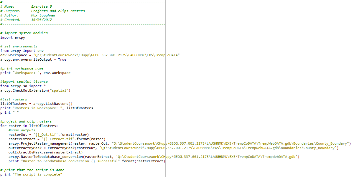
Python Script to Assign Weights to Factors

A Python script was also developed to weight a certain factor in the model. This script can be viewed here under Script 3.


RESULTS AND DISCUSSION

The land suitability factors are shown below in figure 7. A raster was created from each factor as described in detail in the methods section. The darker the area, the better suited it is for a sand mine.

Figure 7: Land suitability factors
These factors were added together to create the raster shown below in figure 8. The darker areas are more suitable for mines. Notice the flat, lightly colored areas, primarily along the southern edge. These are the areas that were excluded.

Figure 8: Sum of suitability factors


Next, the negative impact factors are shown below in figure 9. The darker the area, the more negative the impact for that area is.

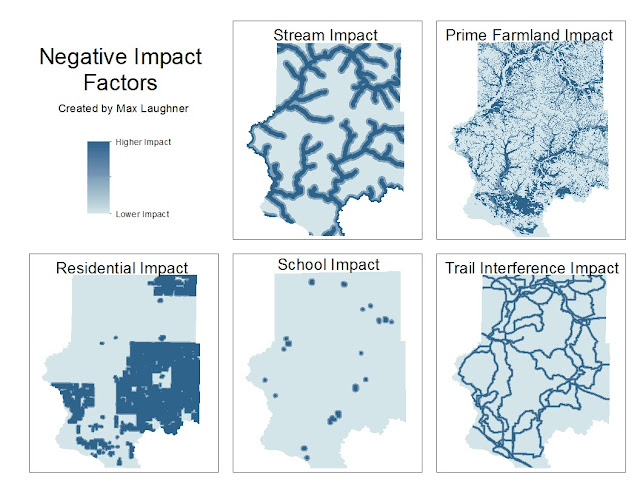
Figure 9: Negative impact factors
Shown below in figure 10 is the sum of the impact factors. Darker areas have higher environmental and social impacts, so the lighter the area, the better it is for a mine.

Figure 10: Sum of impact factors

Finally, the map created for recommended mine locations is shown below in figure 11. This takes into account the previously discussed factors for successful mine locations along with areas of negative environmental and social impact. Many areas on the southern portion of the county are inadvisable as mine locations. This is due to those areas being part of the river or state park area. Lines of excluded areas throughout the map show rivers and major roadways that are surrounded by developed land. The best locations found for potential sand mines are largely in the western side of the county. There are also many areas of high rank scattered in the southern area.

Figure 11: Recommended areas for sand mines


CONCLUSION

Raster analysis functions are a robust option for data analysis. The Raster Calculator tool, while simple, is vital in connecting multiple data sets. The multitude of raster analysis tools available are vital to any raster-based application. While some factors were simplified for the purpose of this lab, real-world workflows are similar to the workflow followed throughout the exercise.


Friday, April 21, 2017

Network Analysis

GOALS AND OBJECTIVES

This lab explores network analysis tools. Network analysis uses networks, in this case road networks, to model routes, distances, and travel times. Whereas traditional analysis uses straight lines, "as the crow flies" routes, from one point to another, network analysis can more accurately analyze how far and how long it takes to travel between points. The tool has a wide range of applications, from routing emergency vehicles on the quickest path, to modeling waterway networks, to finding travel routes around construction zones. Applications of this network analysis are widespread.

In this lab, the sand mine data used previously will be studied here. The goal of this lab is to find hypothetical costs associated with road wear caused by heavy mining vehicles using public roads. To do this, routes must be established that the vehicles will take, then the distance of these routes needs to be determined, followed by the total cost calculated from this distance.


METHODS

This lab began with a Python script (can be viewed here under script 2) that used SQL queries to find mines that would need to use roadways to transport frac sand. This was done by removing deactivated mines and mines that are connected to a rail terminal. Next, the script used a select by location to remove mines that were 1.5 km from a rail terminal, as these would have spurs built that would eliminate the need for roadway transport. The script was run and the relevant mines were extracted successfully.

These mines were then brought into ArcMap, along with rail terminal locations and road network analysis features. To minimize error, the network analysis was then done with a model. This model is shown below in figure 1. The three inputs: streets, mines, and rail terminals were used in the network analysis tool to find the closest route from each mine to a rail terminal. These calculated routes were copied and exported to a new feature class. A map showing these routes can be seen in the results section.

Figure 1: Model created for network analysis

Next, a model, shown in figure 2, was used to estimate the hypothetical cost that vehicles using the routes would incur on roadways. The cost was estimated per county. First, in the model, the routes were projected to a Wisconsin HARN projection to minimize distortion. next, the routes were cut along county lines with the identity tool. This was done so distance calculations within counties would be limited to sections of routes that fall within the county. The identity tool added fields to the routes that had data on which county each section of the route was in. The summary statistics tool then merged all route sections by county to determine total distance of route in each county. Add and calculate field tools were then used to take this distance, convert it into miles, multiply this by a hypothetical cost of 2.2 cents per mile and 50 trucks making a round trip per year. The numbers used are hypothetical and could be easily changed by altering variables in the model.

Figure 2: Model created to estimate cost per county for road usage


RESULTS AND DISCUSSION

Shown below in figure 3 are the routes that were predicted from each mine a rail terminal. Notice there are some rail terminals that connect to multiple mines. Also, overlapping routes are still considered to be separate routes, so distance is calculate individually per route. This is why, as will be shown in the cost calculations, counties with a dense network of routes have a higher predicted cost than counties with a single, long route.

Figure 3: Routes from mines to rail terminals

Below in figure 4 is a chart showing estimated costs per county. This was created by exporting the table created by the second model to Excel. There are many counties with negligible calculated costs as a route only briefly passes through. The counties with the highest costs have dense networks of predicted routes. The calculated costs for roadway wear were relatively low compared to the scale and cost of sand mine operations. Of course, the cost per mile, one of largest factors, was just a hypothetical estimate in this exercise and the actual cost per mile could be much higher or lower.

Figure 4: Chart showing hypothetical yearly costs per county

Lastly, shown in figure 5 is a map depicting estimated costs by county.
Figure 5: Map showing hypothetical yearly cost per county
The best way to mitigate these costs would be to ensure there are rail terminals close to areas of high mine concentration. With many mines in Chippewa county, the highest cost county near the center, a rail terminal could be build near the center of the cluster to greatly reduce mine-to-rail distance.

There are many assumed variables that cause uncertainty in this estimation. Beyond the hypothetical values used for estimating cost, the method of analyzing routes should be considered. The model chose the route that takes the least amount of time. This may not be accurate, as in reality, routes would also be directed away from high-traffic areas, along with other factors. These factors can be assessed with the network analysis tool with access to pertinent data.


CONCLUSION

Network analysis is a robust tool with widespread applications. Despite this, the tool is relatively easy to use and adapt to fit the application. As shown in this lab, the results from the tool can easily be used in conjunction with other tools as needed. While specialized uses for network analysis, such as cost estimations, are common, even more common is its use in personal routing. Entering a location into Google Maps, for example, uses network analysis to determine the most efficient routes to take. The usefulness of network analysis cannot be stressed enough.


Friday, April 7, 2017

Data Normalization, Geocoding, and Error Assessment


GOALS AND OBJECTIVES

The goal of this lab was to explore geocoding. Geocoding involves using software to match up location descriptions, such as addresses, to actual coordinates on the Earth's surface. In order to geocode, the data had to be sufficiently normalized. This was done by manipulating tables to create similar data for each entry in the table. After geocoding and manual cleanup, error assessments were made to analyze the success of the process.

This lab served as a continuation of the previous frac mining labs. This meant that the data used was frac mine locations, whose locations were given as addresses or described with PLSS. The results from this lab will be used in subsequent labs using network analysis.


METHODS

Before the data could be used in any meaningful way, it had to first be normalized. The goal of normalization is to have a uniform style of data entry so data could easily be compared and analyzed. The initial spreadsheet used is shown below in figure 1. All the location data is given in a single column. Notice the variety of location descriptions. There is PLSS descriptions mixed with addresses. Some have both or only one, and there is no uniform method of entry.

Figure 1: Data before normalization
To normalize the data, entries were split into separate columns: an address column and a PLSS column. This is shown below in figure 2. The geocoding software uses addresses only, so PLSS data would just be for manual cleanup after the geocoding had been run.

Figure 2: Data after normalization
With the data normalized, it was ready to be geocoded. The spreadsheet was brought into the geocoding tool on ArcMap. This tool analyzed the address and town fields to find possible matches for locations. This could only be done on entries with addresses given. For entries with only PLSS locations, the estimated location was automatically chosen at the center of the given town. A visual of this process is shown below in figure 3. First the PLSS township was found, as shown on the right. In this example, the PLSS township was 33 N 13 W. Next, the subsection was used, as shown in the middle. This mine was described as being on the border of section 29 and 32. The area was searched for a mine and found, as shown on the right. The location, as marked by an X, was placed on the road to ease in network analysis for future labs.

Figure 3: Using PLSS data to find mine locations
This was done for all mines with PLSS data. All other mines were similarly checked to make sure the location was marked at the entrance of the mine. Many of these were off and had to be manually corrected, as the geocoding software uses approximations to guess locations for addresses.

For error analysis, the data was compared to both the class's data and the coordinates given by the data provider. Comparisons were made in a similar way for each. For comparisons to student data, all mine shapefiles were merged into a single feature class and projected in in Central Wisconsin State Plane projection. The lab was designed so there was overlap enough so each mine was located by several students. This meant the feature class had multiples of the same mines. Once this feature class was created, a model was made to split each unique mine into separate feature classes. This model is shown below in figure 4. The model iterates through the feature class containing all mines and groups mines with the same mine ID into their own feature classes, naming each output file by the unique mine ID. This was done so each student mine locations could be compared to the corresponding mine location I found. These distances would be averaged to find average distances between my mines and mine locations found by others.

Figure 4: Model created to split unique mines into separate feature classes
This same process of splitting to individual mines was used to the shapefile of actual mine locations given by the DNR. In this case, however, there was a one-to-one ratio of mines being compared, as I was not using data from multiple people.

After error analysis was completed, maps were created showing the comparisons of mine locations I found to locations found by other students and to those given by the DNR.


RESULTS

The error calculations performed are shown below in figure 5. Notice there are many more mines being compared under student mines because there were several instances of each mine compared. The averages, or average distance between my mine and other mines, were both around 1700 m.

Figure 5: Error calculations

Shown below in figure 6 is the map created comparing my mine locations to those of other students. Notice that many mines overlap, some completely. There are some outliers, however. Most of these are from a student choosing the wrong mine in the area.

Figure 6: Comparison of my mine locations to those found by students
Shown below in figure 7 is the comparison of my mines to the "actual" locations given by the DNR. I hesitate to call them that because many of these DNR locations have low precision, and are placed a distance from where the mine is clearly located on aerial imagery. This is a cause of higher error found previously.

Figure 7: Comparison of my mine locations to those given by the DNR


DISCUSSION

Using the model turned out to be an excellent way to efficiently split feature classes for easier use. Doing this allowed me to compare all mines available rather than taking a sample and only comparing 10 or 20 percent of the mines.

There are a few sources of error that make the average distances non-zero. One is that not all mines analyzed are active. Some mines are closed and reclaimed as vegetated areas, with makes their precise location difficult to assess. For these, maps from different temporal resolutions were used. Some mines, however, were only permitted and construction had not yet begun. There was no real way to find precise locations on these, so locations were marked near open areas away from private residences. There were some mines that were found, but were large and had multiple entrances. This resulted in the lower end averages that are seen, as some students picked a different entrance than I. There were some instances of choosing the wrong mine, as some areas have a high density of mines and only have a vague PLSS description of the mine location, resulting in ambiguity of which mine is the correct one.


CONSLUSION

Geocoding is a powerful tool that is used by almost everyone. Typing an address into Google to find its location is an example of how geocoding is used in every day life. Geocoding as an analysis tool proved to be extremely useful, but not without its shortfalls. A significant amount of time was spent checking and correcting mine locations from either incorrectly estimated locations or the inability for the software to use PLSS location data. Nevertheless, the geocoding software has impressive abilities that become most useful when dealing with a large number of data entries. The amount of time it takes to locate entries with geocoding software is a fraction of the time it would take manually.


Monday, March 13, 2017

Gathering Data for Trempealeau County

GOAL AND OBJECTIVES

The goal of this lab was to gather data from online sources and import the data into a single geodatabase. This was done largely through a Python script designed to project and clip the data while importing it into the geodatabase. The study area for this lab was Trempealeau County and is a continuation of the previous lab's focus on frac sand mining in the county.

The data came from a variety of online sources. This included DOT railroad data, USGS land cover and DEM data, USDA cropland data, Trempealeau County land records, and USDA NRCS soil data. The Trempealeau County land records contained a geodatabase for the county, which was used as the main geodatabse for the lab.


METHODS

The basic workflow is as follows:

First a workspace had to be created. Since a large amount of data would be downloaded, a temporary working folder was created to store the files until they were processed and put into a geodatabase.

Next, the data was downloaded. First, the USGS data was obtained. This was done by navigating to the USGS National Map Viewer, selecting Trempealeau County, and downloading the National Land Cover and DEM data. Next, the USDA website was used to download the land cover data. Next, the Trempeleau County Land Records geodatabase was downloaded from the website. This would serve as the main geodatabase for the project. Lastly, the USDA NRCS Web Soil Survey data was downloaded from the USDA website.

The data, all kept in the working folder, was then unzipped to allow it to be used. The geodatabase was moved to the project folder to serve as the main geodatabase. The USDA Soil Survey data was then imported to the geodatabase after joining the tabular data into the shapefile using a Microsoft Access macro. Next, the railroad data was processed. Since this shapefile expanded beyond the scope of Trempealeau County, it was clipped to the county and imported to the geodatabase. Importing it into the feature dataset automatically projected it into the correct Trempealeau County projection.

Next, a Python script was written to project, clip, and import the raster data into the geodatabase. This included the NLCD, the USGS DEM, and the NASS data. The Python script is shown in the blog post about scripting, under Script 1. This script was designed to loop through every raster in a given folder and project it, clip it to Trempealeau County, and import it into the geodatabase.

Lastly, the rasters were used to create a map of Trempealeau County in ArcMap. This is shown in the results section.


RESULTS

Shown below in Figure 1 is the map created from the raster files. The legend for the NASS and NLCD maps have a large number of categories, so they are shown separately below in Figure 2.

Figure 1: Map created from raster data for the county

Figure 2: Legends for the map above

Shown below in figure 3 is a table showing the data quality for each dataset used. This information was obtained from the metadata for each set. Notice there are many values enetered as "NA." This means the information could not be found in the metadata or this did not apply for this dataset.

Figure 3: Data quality for each dataset used

CONCLUSION

This lab gave an introduction to basic data gathering from a variety of sources, as well as some Python scripting. The emphasis in this lab was data quality assessment. It is obviously important to know how to download data, but more important than that is being able to assess the quality of the data, otherwise results will be invalid.


Friday, March 10, 2017

Python Scripts

BACKGROUND

Python is an Integrated Development Environment, or IDE, that allows users to write code, debug, and run it. Scripting is useful when doing repetitive work. Writing a script instead of doing repetitive scripts multiple times can minimize the amount of time it takes to carry out tasks and can minimize room for error.


GOAL

The goal is to learn basic Python scripting and be able to implement it in future work. These scripts should obviously be functional, but also important is that they are well commented so other users can easily understand them.


SCRIPTS

Script 1:


This script projects and clips all rasters within the workspace geodatabase.


Script 2:
This script runs several SQL queries on a vector and saves the results.


Script 3:


This script assigned rasters to variables, weights a variable, and adds them. The result is then saved.


Thursday, March 2, 2017

Background on Sand Mining in Western Wisconsin

OVERVIEW

What is frac sand mining?

Frac sand is used for injecting into oil and gas wells under high pressure to enlarge fractures and create new ones. The fluid is then pumped out. Frac sand mining is the process of extracting this sand from the ground. The sand needed for this process must be of round, uniform size, quartz sand which is found in abundance in Western Wisconsin.


Where is frac sand found in Wisconsin?

The sand is taken from sandstone formations, which spread across Western Wisconsin. Below (Figure 1) is a map taken from the 2012 Wisconsin Geological and Natural History Survey. This shows the spread of sandstone across Wisconsin. Notice how it is spread densely across the Central and Western side of the state. This distribution is caused by glacial deposits and results in round sand of a size perfect for industrial applications. There are other deposits in the Southern and Eastern side of the state, but these grains tend to be smaller and more angular, which is less useful for industrial applications.

Figure 1: Locations of sandstone formations across Wisconsin

What are some of the issues associated with sand frac mining in Western Wisconsin?

The magnitude of the environmental impact varies greatly depending on the type of operation and the location. Common impacts are described below.

Frac sand mining produces a significant amount of air pollution. This is from two sources. The first is dust that is released during the blasting process and the subsequent handling of the sand. The second is from the machinery used to extract and process the sand, such as extraction equipment, generators, pumps, heavy transportation vehicles, and more.

Water pollution is also a result of the process. This is more site-specific than air pollution. Water pollution is created from several sources, including cleaning, transportation, dust control, and sorting. These can contaminate water with industrial chemicals and affect the availability of water for nearby wells.

Another impact of the mining is the effect it has on the land surface. Reaching and extracting the sand requires vegetation to be removed, which affects wildlife habitats. A reclamation process is possible on some mines after they are closed, but this process is difficult and expensive. Noise is also a problem during the process, which similarly affects local wildlife.

Traffic from transportation equipment is also a concern. These heavy transportation vehicles causes significant wear on roads and can be a burden by blocking local traffic.


How GIS will be used to further explore these issues

GIS can be used to study how certain areas will be impacted by sand mines. Environmental data including wildlife, water, air quality, and climate data can be used to predict possible impacts. For example, fish habitats could be compared with likely water pollution scenarios to determine how the habitat will be affected. Climate data could also be assessed to determine where and how far the air pollution from mines would travel.

Non-environmental impacts can also be studied. The wear of roads could be predicted along with traffict impacts. Noise pollution could also be predicted for those living nearby a mine.

GIS systems are critical to predicting impact of virtually every aspect of sand mines. This data can be used to find optimal locations for these mines to minimize negative impacts.


SOURCES

Brown, Bruce. "Frac Sand in Wisconsin." Wisconsin Geological and Natural History Survey (2012): n. pag. Wcwrpc.org. Web.

Pearson, Thomas W. "Frac Sand Mining in Wisconsin: Understanding Emerging Conflicts and Community Organizing." Culture, Agriculture, Food and Environment 35.1 (2013): 30-40. Wisconsin DNR. Jan. 2012. Web.

Kremer, Rich. "Is Frac Sand Mining Causing Metal Contamination In Groundwater?" Wisconsin Public Radio. N.p., 14 Oct. 2016. Web. 02 Mar. 2017.